SolidWorks Closed Loop Control Simulation
Modeling real life system into Solidworks for a close loop control and vibration analysis
May 1st, 2023
Nathan Sun
.png)
Figure 1. The Real Life System
Background
The purpose of this simulation is to convert a real life multibody dynamic system into a SolidWorks simulation, and study its various properties including displacement, friction force, and vibrations between parts. As shown in Figure 1, the real life counterpart to the simulation has a rotating shaft that has neoprene rubber attached on it, a cantilevered AISI 1020 beam with the same rubber on its end is pressed against the shaft, while the two rubber make contact and the beam oscillates up and down due to rubber's high friction.
Deliverable 1: Multibody Dynamic Model
Reproducing a stick-slip friction behavior exhibited by neoprene rubber block and shaft when under force.

Figure 2. Refraining Planes to the Block
.png)
Figure 3. Neoprene Rubber Properties
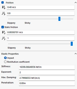
Setup: To simulate the real life system, many assumptions must be made, and the simulation system can also simplify many scenarios. The neoprene rubber block is limited by three planes shown on the left, making it only able to move vertically and inwards/outwards against the shaft, as seen in Figure 2. The properties of the neoprene rubber include dynamic friction coefficient of 0.8, static friction coefficient of 1, elastic exponent of 2, and 0 inch penetration (shown in Figure 3.).

Figure 4. Spring Simulation Setup to the Block
A spring, simulating the vibration of the long beam shown in Figure 1., is placed under the block by two reference points, with its spring constant K calculated and analyzed in Deliverable 2. This setup is presented in Figure 4.
.png)
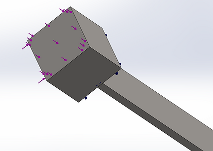
Figure 5. Force Applied to the Block
A chosen force of 1lbf (Figure 5.) will be pushing the neoprene block into the shaft as it rotates (shown in Deliverable 3).
Deliverable 2: Finite Element Model of a Prismatic Beam
Finding a theoretic spring constant of a cantilevered beam and comparing it to the ideal value.
An AISI 1020 beam with dimensions of 12 in.*1 in. * 0.125 in. is held still on one end by fixtures, while the other end is applied with a force of 0.25 lbf (Figure 6). After applying SolidWorks static force simulation, as shown in Figure 7, its vertical displacement can be found as 0.003028 inches.
.png)
Figure 6. The fixture and the Force Applied to the Beam

Calculations are then made to compare the values of K due to simulation displacement, and K due to material property and geometry.
As shown in Figure 8, the % error is minor at only 0.739%, indicating the experimental value K at 8.256 lbf/in. is an ideal estimation of the system when the beam is considered as a spring in Deliverable 1 and future use.
Figure 7. Simulated Displacement

Figure 8. Spring Coefficient Constants Calculations
Deliverable 3: Constant and Closed Loop Speed Control
Analyzing shaft rotation in constant speed and close loop controlled speed and comparing the differences.

To fully study the motion and interaction of the system, rotation of the shaft is to be added. There will be two ways of rotation added to the shaft, one by constant rotating speed of a motor at 30 rpm, and the other by applying a closed loop controlled variable rotational speed motor.
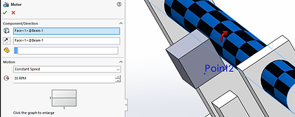
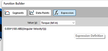
Figure 9. Constant Speed Settings
Figure 10. Closed Loop Calculation Parameters
Figure 9 shows the applied direction and speed of the rotation at 30 rpm of the motor on the shaft, and Figure 10's parameters are acquired by obtaining a rotational velocity of the shaft at constant speed, and applying that data into the closed loop. The expression is 0.04*(180-ABS({Angular Velocity1})), where 0.04 is the constant for a study velocity and torque output, and Angular Velocity1 being the rotational velocity mentioned previously. It was used to adjust the torque output, which will be increased when it sees a decrease of velocity due to larger friction (Observed in Figure 11a, further explained down below)
Angular Velocities
Case A: Constant shaft rotational speed at 30 rpm
Case B: Closed loop controlled speed
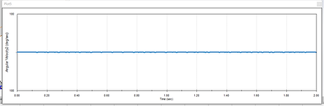
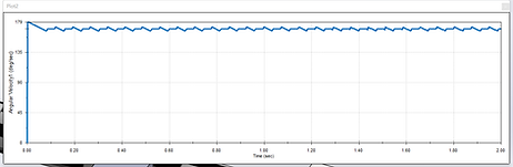
Figure 11a. Angular Velocity at 30 rpm
Figure 11b. Angular Velocity at Closed Loop
Comparing the angular velocities between constant speed and closed loop speed at Figures 11a and 11b, it can be observed that the constant rotational speed at 30 rpm's shape is a flat line over time, with slight fluctuations from time to time, this makes sense because although the motor wants to maintain at 30 rpm, while the friction force resist against the motor, causing unwanted slow downs in rotational speeds and hence the fluctuations observed.
On the other hand, different than the constant speed case, the angular velocity of the closed loop quickly raises to a maximum value and slighly dips down to an oscillating angular velocity. This corresponds to the slipping of the neoprene rubber as the shaft rotates, the closed loop compensates for the larger friction force by spinning at higher speeds.
Motor Torques
Case A: Constant shaft rotational speed at 30 rpm
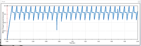
Figure 12a. Motor Torque at 30 rpm
Case B: Closed loop controlled speed

Figure 12b. Motor Torque at Closed Loop
If closely compared in Figure 12a and 12b, the oscillating portion between constant speed and closed loop speed are highly identical (visually different due to graph scales), this is due to the fact that motor in both cases withstand the same frictional forces as the shaft rotates, hence outputting similar amounts of torque and curves over time.
The difference lies in the beginning, as the torque of constant speed starts from 0, while the torque of closed loop drop from a higher value before entering the oscillation. The reason behind the torque drop of closed loop controlled motor is due to its need to constantly sense the force and make adjustments through its PID controls, if starting from 0, it may have trouble in the first few seconds to affectly adjust for the changing forces, but the constant 30 rpm motor does not need to have such a need to sense from the beginning due to the lack of PID controls.
Deliverable 4: Beam Vibration
Finding and making sense out of the vibrations found in both realistic simulation modeling and block simulation modeling
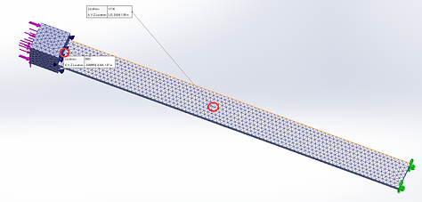
Figure 13. Block-Beam System Simulation
.png)
Figure 14. Vibration Results at Midpoint and End of Beam
In deliverable 4, the simplified block-spring system was replaced by a block-beam system (Shown in Figure13.), which is closer to the real-life system. The real time friction force simulated in the block-spring system is used to be the direct output to the new block-beam system, leading to results including peak amplitudes, main frequencies, which can also be compared to those results in the block-spring system for accuracy validation. The vibration properties of the block and beam system is studied at two nodes, namely one at the middle of the beam, and the other at the end of the beam, as highlighted in Figure 13, and their displacement results shown in Figure 14, with the blue data line showing the center node.
.png)
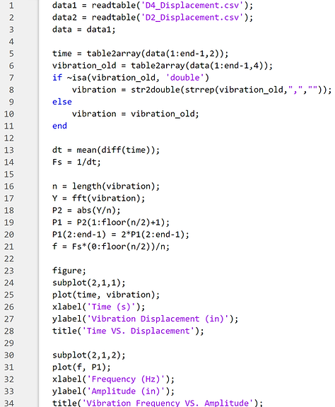
Figure 15. Two Forces to the System
Figure 16. MATLAB Code to Show Displacement and Frequencies
Code Created in Collaboration with Qiu, Peng
The study is done by a SolidWorks linear dynamic study, which has the beam cantilevered at one end, the block and beam connected under rigid connections, one constant force set against the block, and one curve varying force (using the friction force data) going upwards against the block, as shown in Figure 15.
After simulation study, the time response graph of the y axis displacement, representing the vibration, was extracted and analyzed using MATLAB codes shown below, outputing results that is further analzed. The code uses Fast Fourier Transform to study the vibration, finding corresponding frequency and amplitude results.
Peak Amplitude of Vibration
1) The peak amplitude of the vibration, simulated in the beam & block simulation using linear dynamic study and friction force results, is 0.123-(-0.054)=0.177 inches, calculated by subtracting the largest vibration displacement to the smallest (Values acquired from Figure 17).
.png)
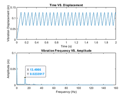
Figure 17. FFT Output of the Block-Beam System's Vibration
Main Frequency & Amplitude of Vibration
2) Shown on the lower graph on Figure 17. is the main frequency at 13.13 Hz, with the amplitude of 0.0532 inches, represented by the highest peak of the Frequency VS. Amplitude graph.
Beam Vibration Compared with Block Vibration
.png)
.png)
Figure 18a. Beam Vibration by FFT
Figure 18b. Block Vibration by FFT
3)Figure 18a. shows the beam's vibration at the node located at middle of the beam, where it is the best location to find the vibration properties of a beam; while Figure 18b. is acquired by inputting the Block-Spring system's displacement data into the FFT analysis. The block-spring system can represent the block because it has excluded the beam, eliminating any possible beam vibration's effects to the block.
The vibration of the beam is similar to that of the block's. Under FFT calculations and observed in Figures 18a. and 18b., the beam shows a main frequency at 13.131 Hz, while the block shows 13.499 Hz, which are close values. The amplitudes are slightly differnt due to geometry differences, with the beam at 0.053 inches and the block at 0.023 inches. Overall they share similar properties of vibration, while maintaining differing displacement profiles.
Beam Vibration under Different Motor Speeds
.png)

Figure 19a. Beam Vibration at 30 rpm Closed Loop
Figure 19b. Beam Vibration at 60 rpm Closed Loop
.png)

Figure 20a. Block Vibration at 30 rpm Closed Loop
Figure 20b. Block Vibration at 60 rpm Closed Loop
4)To find out the difference in vibrations under different motor speeds, another set of simulation, with closed loop control set at 60 rpm was conducted, as shown in Figure 19b. and Figure 20b. Both beam and block behavoirs was found to be similar. For Beam vibration, the main frequencies remained the same at 13.13 Hz, while a diminutive difference of amplitude at 0.053 inches and 0.063 inches were shown. For Block vibration, the main frequencies between 30 rpm and 60 rpm are slightly different, with 13.50 Hz for 30 rpm and 16.00 Hz for 60 rpm, while the amplitudes are similar at 0.0234 inches and 0.0285 inches. Hence, it is safe to conclude that different rotational speeds of the motor, for both beam and blocks do not affect the vibration properties, namely the main frequencies and the amplitudes.